Jin Hyun Park / Qual Exam Prep / Algorithms

Algorithms and data structures

The largest part of the exam. Most questions ask for a running time, a property, or which algorithm applies.

Hash tables

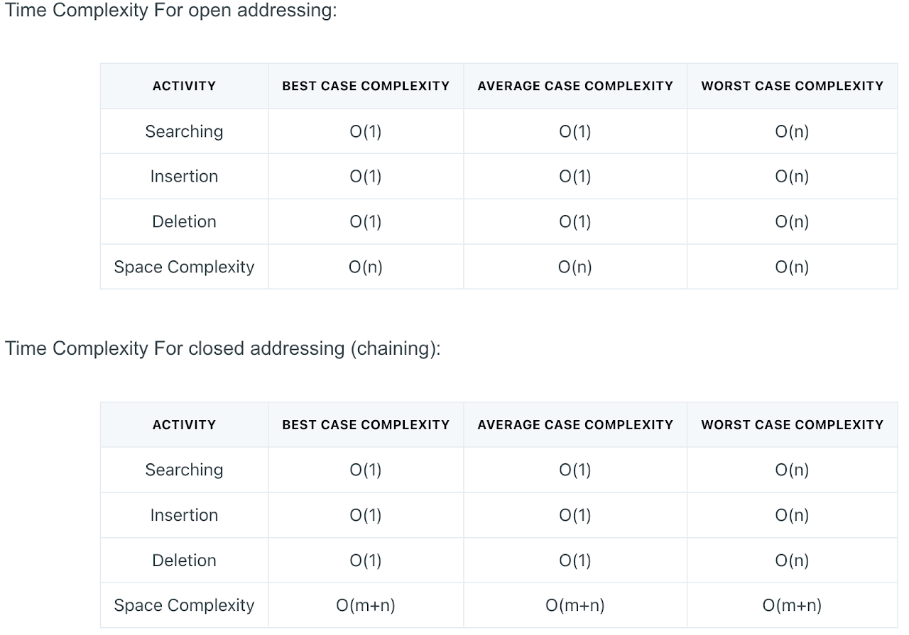
• A hash function maps each key to a slot. A collision is when two different keys map to the same slot, and every hash table needs a way to deal with it (GeeksforGeeks).
• Chaining (closed addressing): each slot holds a linked list, and colliding keys are simply appended to the list.
• Open addressing: everything stays in the array. On a collision, a rule picks another slot to try: linear probing (try the next slot), quadratic probing (try slots 1, 4, 9, … away), or double hashing (the step size comes from a second hash function).
• Either way, search, insert, and delete are O(1) on average and O(n) in the worst case, when everything lands in the same slot.

BFS and DFS

• Both visit every vertex and every edge once, so both run in O(V + E) with an adjacency list.
• With an adjacency matrix, finding the neighbors of a vertex means scanning a whole row, so the time becomes O(V²).

Topological sort

• Orders the vertices of a directed acyclic graph (DAG) so that every edge points from an earlier vertex to a later one. Think of tasks with prerequisites.
• Method (Kahn's algorithm): repeatedly take a vertex with no incoming edges, output it, and delete it along with its outgoing edges. If you run out of such vertices before the graph is empty, the graph has a cycle.
• Time: O(V + E).

Shortest paths

• Single source: shortest paths from one vertex to all others (Bellman–Ford, Dijkstra).
• Single pair: from one vertex to one other vertex. In practice you run a single-source algorithm and stop early.
• All pairs: between every pair of vertices (Floyd–Warshall, Johnson).
• Useful fact: any sub-path of a shortest path is itself a shortest path. This is the optimal substructure that all of these algorithms rely on.
• The longest path problem is NP-hard in general, but on a DAG it is easy: process the vertices in topological order.

Bellman–Ford

• Not greedy. It relaxes every edge, and repeats that V − 1 times.
• Works on directed and undirected graphs, and handles negative edge weights as long as there is no negative cycle (Baeldung). It can also detect a negative cycle: if a V-th round still improves something, there is one.
• In an undirected graph a negative edge is a negative cycle (go back and forth along it), so negative weights are only meaningful in directed graphs.
• Time: O(VE), which is O(V³) on a dense graph.

Dijkstra

• Greedy: always settle the closest unsettled vertex next.
• Works on directed and undirected graphs, but assumes no negative weights. With negative edges the greedy choice can be wrong.
• When both apply, Bellman–Ford and Dijkstra give the same answer; Dijkstra is just faster.
• Time: O(V²) with a simple array, or O((V + E) log V) with a binary min-heap.

Floyd–Warshall

• Dynamic programming over "paths that only use the first k vertices as intermediates".
• Works on directed and undirected graphs, and on directed graphs it tolerates negative weights (but not negative cycles).
• Produces the shortest path length between every pair of vertices.
• Time: O(V³), regardless of how many edges there are.

Johnson's algorithm

• Also all-pairs. It reweights the graph with one run of Bellman–Ford so that Dijkstra can be run from every vertex.
• Faster than Floyd–Warshall on sparse graphs (few edges). For the exam, knowing that much is enough.

Minimum spanning tree (MST)

• A spanning tree of a connected graph is a connected, acyclic subgraph that includes every vertex. With n vertices it always has exactly n − 1 edges.
• The minimum spanning tree is the spanning tree whose edge weights add up to the least. Think of connecting cities with the cheapest possible set of roads.
• It is defined on undirected, weighted graphs. The MST is not necessarily unique (ties in edge weight can give several), but its total weight is.
• Generic algorithm: start with an empty edge set A; repeatedly add an edge that is "safe" (keeps A a subset of some MST); stop at n − 1 edges. Kruskal and Prim are two different ways to pick a safe edge.
• Kruskal's algorithm (greedy, edge-based)
  1. Sort all edges by weight.
  2. Go through them in order and keep an edge unless it would create a cycle with the edges already kept (use a union-find structure to check).
  3. Stop after n − 1 edges.
  Time: O(E log E) = O(E log V), dominated by the sort.
• Prim's algorithm (greedy, vertex-based)
  1. Start from any vertex.
  2. Grow a single tree outward.
  3. At each step add the cheapest edge that connects a vertex in the tree to one outside it.
  Time: O(E log V) with a binary heap, O(V²) with a plain array (which is fine for dense graphs).
• Prim and Kruskal always agree on the total weight, but they may pick different edges when there are ties.

Tree traversals

• Walk the tree recursively, and imagine you pass each node three times: once on the way down, once between its children, and once on the way back up.
• Pre-order: output the node the first time you pass it (node, left, right).
• In-order: output it the second time (left, node, right). On a binary search tree this gives the keys in sorted order.
• Post-order: output it the third time (left, right, node).
• The clearest explanation I have found is this video.

Dynamic programming

• Step 1: write a recurrence that expresses the answer to a problem in terms of answers to smaller subproblems.
• Step 2: solve it without recomputing the same subproblem over and over, in one of two ways:
  • Top-down with memoization: write the recursion naturally, but cache every result. Only the subproblems actually needed get solved.
  • Bottom-up: fill a table from the smallest subproblems upward. No recursion, so no function-call overhead.

Optimal substructure

• A problem has optimal substructure if an optimal solution can be built from optimal solutions to its subproblems. Shortest paths have it; longest simple paths do not.
• Greedy algorithms and dynamic programming both depend on it. Dynamic programming additionally needs overlapping subproblems; greedy algorithms additionally need the greedy-choice property.

Recursion

• What keeps a recursive function from running forever? Think of the Fibonacci numbers.
  • Base case: at least one input for which the function returns without calling itself (fib(0) and fib(1)).
  • Recursive case: every recursive call must move toward the base case (fib(n) calls fib(n − 1) and fib(n − 2)).
• Put differently: a recursive function must have an execution path on which it does not call itself, and it must have something (a parameter or a global variable) that changes between calls so that the base case is eventually reached.

2-SAT vs. 3-SAT

• 2-SAT (each clause has two literals) is in P; it reduces to finding strongly connected components in an implication graph.
• 3-SAT (three literals per clause) is NP-complete. It is the standard starting point for NP-hardness reductions.

P, NP, NP-hard, NP-complete

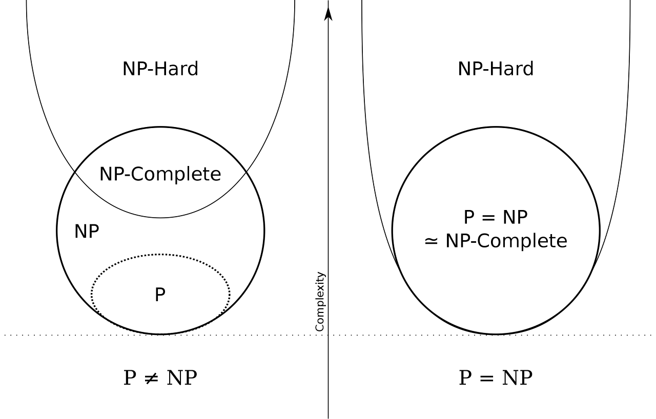
• P (polynomial time): problems a deterministic machine can solve in polynomial time. Sorting, shortest paths, 2-SAT.
• NP (non-deterministic polynomial time): problems a non-deterministic machine can solve in polynomial time. Equivalently, problems whose "yes" answers can be verified in polynomial time if someone hands you a certificate. P ⊆ NP.
• NP-hard: at least as hard as every problem in NP. Formally, X is NP-hard if every problem in NP can be reduced to X in polynomial time. NP-hard problems need not themselves be in NP (the halting problem is NP-hard but not in NP).
• NP-complete: in NP and NP-hard. These are the hardest problems in NP. 3-SAT, clique, Hamiltonian cycle, graph coloring.
• How reductions are used:
  • To prove A is NP-hard, take a known NP-hard problem and reduce it to A (not the other way round).
  • If Q is NP-complete and Q reduces in polynomial time to R, then R is NP-hard, and therefore R is not in P unless P = NP.

Depth and height of a tree node

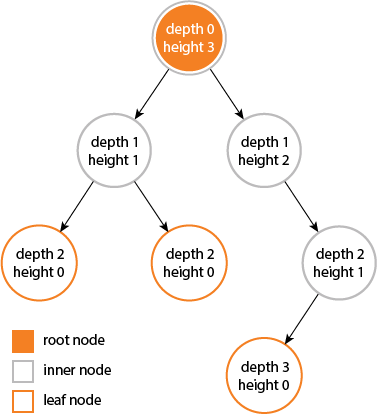
• Depth is measured from the root: the root has depth 0, its children depth 1, and so on.
• Height is measured from the leaves: a leaf has height 0, and a node's height is one more than the height of its tallest child. The height of the tree is the height of the root.

Maximum flow

• Max-flow algorithms are not greedy: they repeatedly find an augmenting path in the residual graph, and a later path may undo part of an earlier one.
• Ford–Fulkerson
  • The general method: repeatedly find any augmenting path (DFS is the usual choice) and push flow along it.
  • Time: O(E · f) when capacities are integers, where f is the value of the maximum flow. With large capacities and badly chosen paths it can be very slow, and with irrational capacities the basic method may not even terminate.
• Edmonds–Karp (Ford–Fulkerson with a specific rule)
  • Finds augmenting paths with BFS, i.e. always the shortest one.
  • Time: O(V · E²), independent of the capacities.

AVL tree

• A binary search tree that keeps itself balanced: for every node, the heights of its left and right subtrees differ by at most 1.
• Insertions and deletions can break the balance, and it is restored with rotations.
• Because of the balance rule, the height is at most about 1.44 · log₂ N for N nodes.
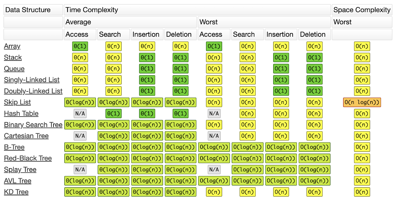
• Search, insert, and delete are all O(log N).

Red–black tree

• Another self-balancing binary search tree. Every node is colored red or black, and the colors follow these rules:
  • The root is black, and every leaf (the NIL sentinels) is black.
  • A red node has only black children (no two reds in a row).
  • Every path from a node down to its NIL descendants passes through the same number of black nodes (the black height).
• These rules guarantee that the longest root-to-leaf path is at most twice the shortest one, which is enough to keep the height O(log N).
• Each node needs just one extra bit to store its color.
• Number of NIL leaves = number of interior nodes + 1.
• Insertion and deletion may require recoloring and rotations. Search, insert, and delete are all O(log N).

B-tree

• A balanced search tree in which each node holds many keys and has many children. It is designed for disk: one node is one disk block, so the number of disk reads is the height of the tree.
• All leaves are at the same depth. Balance is kept by splitting and merging nodes, so no rotations are needed.
• Height ≤ log_t((N + 1) / 2), where t is the minimum degree (the minimum number of children per internal node).
• Search, insert, and delete are O(log N).

Simple graph

• Also called a strict graph: undirected, no self-loops, and at most one edge between any two vertices. Weights are allowed; "simple" is about the structure, not the weights.

Loop invariant

• A statement about the program's variables that is true before the loop starts, stays true after each iteration, and is therefore still true when the loop ends. Proving a loop correct means finding the right invariant.

Singly vs. doubly linked lists

• Search is O(N) for both; you have to walk the list.
• Insertion and deletion are O(1) for both, once you are at the right position (for a singly linked list, that means having a pointer to the node before the position).
• Insertion after node A:
  1. Create the new node.
  2. Point the new node at A's old successor.
  3. Point A at the new node.
• Deletion of B from A → B → C:
  1. Point A at C instead of B.
  2. B still points at C, which is harmless.
  3. Free B.
• A doubly linked list also keeps a pointer to the previous node, so it can be walked backward and a node can be removed with only a pointer to that node.

Common data structures and their time complexities

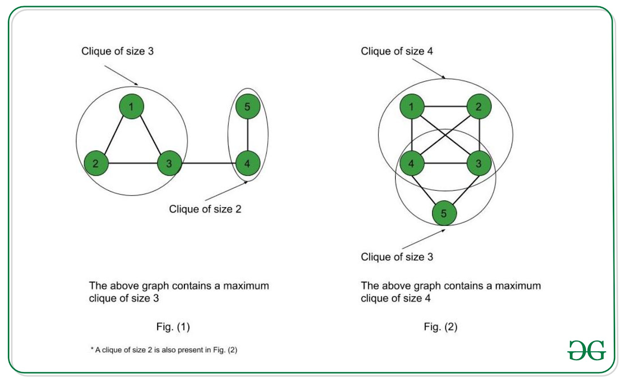
Clique

• A clique is a set of vertices in which every pair is connected by an edge, i.e. a subgraph that is a complete graph.
• The clique decision problem asks whether the graph contains a clique of size k. It is NP-complete.

Eulerian vs. Hamiltonian

• An Eulerian path uses every edge exactly once; an Eulerian circuit does so and returns to the start.
  • A connected graph has an Euler circuit if and only if every vertex has even degree.
  • It has an Euler path (but not a circuit) if and only if exactly two vertices have odd degree; the path starts at one of them and ends at the other.
  • Checking this is easy, so the Eulerian problems are in P.
• A Hamiltonian path visits every vertex exactly once; a Hamiltonian circuit also returns to the start. Deciding whether one exists is NP-complete.

Circuit vs. path

• A circuit is a closed walk with no repeated edges; it starts and ends at the same vertex and may pass through a vertex more than once (an Euler circuit usually does).
• A cycle is a circuit that also repeats no vertex.
• A path does not return to its starting vertex.

Boolean logic

• AND: A · B
• OR: A + B
• NOT: ¬A
• NAND: ¬(A · B) = ¬A + ¬B (De Morgan)
• NOR: ¬(A + B) = ¬A · ¬B (De Morgan)
• XOR: A ⊕ B = A · ¬B + ¬A · B = (A + B) · (¬A + ¬B). True when the inputs differ.
• XNOR: A ⊙ B = A · B + ¬A · ¬B = (A + ¬B) · (¬A + B). True when the inputs are equal.

Overview · Useful materials · Sample questions · Architecture · OS · Networking · Databases · Automata · AI / ML · Things to remember